Deploy and monitor a serverless application > Visualize your data with Kibana

Visualize your data with Kibana

You’ve seen that Kibana provides you with an intuitive search front end for the data in your logs. You can also build visualizations that provide you with monitoring of your underlying infrastructure and application.

The Bookstore app sends data from X-Ray and the Lambda functions themselves. You have set up index patterns for trace segments, and application logs. Let’s pull some information out of that raw data.

A simple visualization: call duration

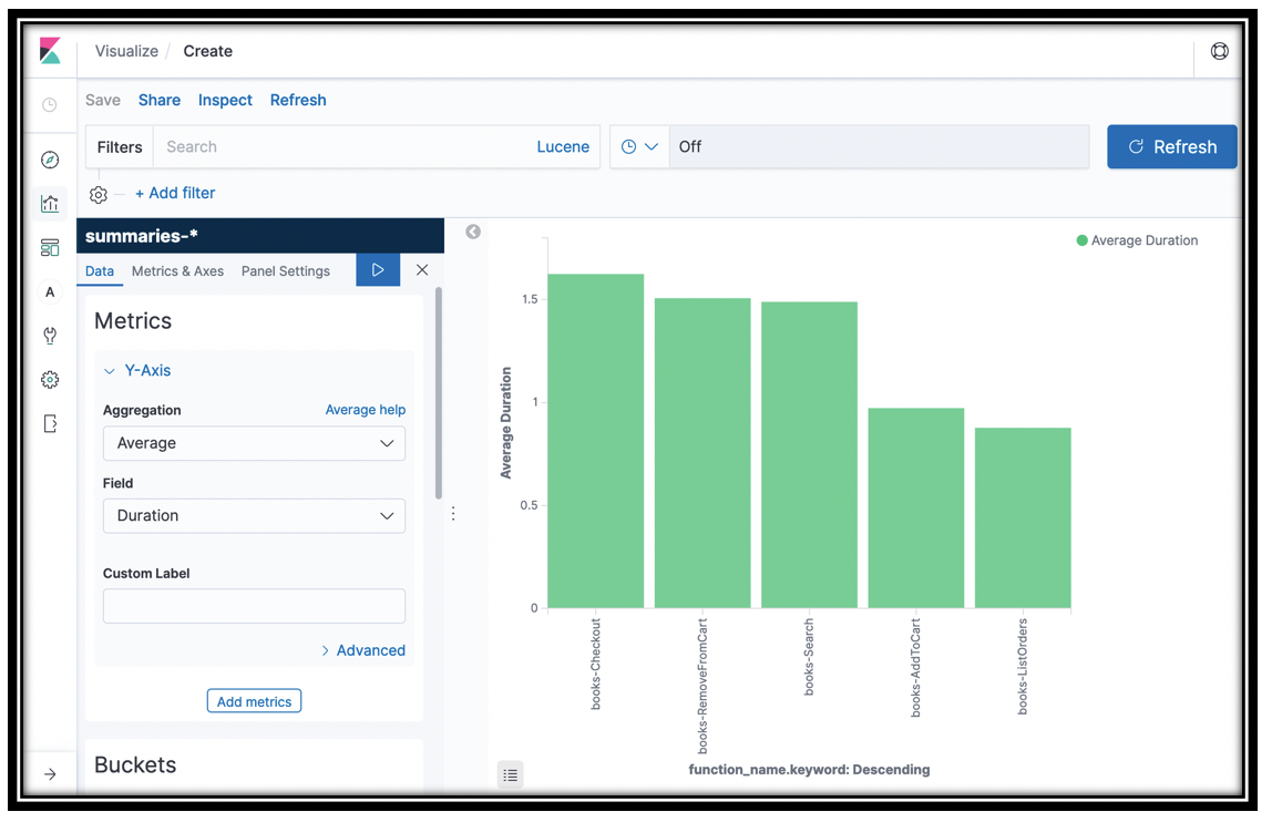
Calls to the Bookstore app come through the API Gateway and are rendered as traces in X-Ray. You can find this data in the trace summaries-* index. The summary data does not have a timestamp, but you can still do some interesting analysis. Let’s visualize the aggregate Duration for each of the Lambda functions.

In the Kibana left navigation pane, click the icon.
Click Create a visualization
In the New visualization dialog, scroll down and click Vertical bar
In the New Vertical Bar/Choose a source dialog, click the summaries-* index pattern.
The visualization panel opens. In this pane you choose the fields to graph on the X- and Y-axes.
In the Metrics section, click the disclosure triangle and select Average from the Y-Axis menu
From the Field menu, select Duration
Under Buckets select X-Axis
Drop the Aggregation menu and select Terms (you might have to scroll the menu to see it)
In the Field menu, choose function_name.keyword
Click the Update icon .

You created a histogram showing you the average Duration for the invocations to your Lambda functions.

Bar chart showing average call duration

We’ll use this visualization in a dashboard in a bit.

Click Save at the top left of the window.
Name your visualization Average lambda duration and click Confirm save

[Optional]: You can add sub-buckets to get a stacked bar chart. Try adding a sub bucket with a Terms aggregation on the ResponseTimeRootCauses.Services.Name.keyword. Or, build a Vertical Bar visualization from the segments index (by selecting the segments-* index pattern when creating the visualization), with a vertical bar for aws_function_name.keyword, with http_response_code (scroll down to the number section of the Field menu) sub aggregation.

Examine the application data

The previous visualization shows some of the power of Kibana. Kibana really shines when working with time-based data like the trace segments and application data. You’re going to build several visualizations for application data and collect those as a dashboard. First you need to understand what’s in that data.

You could use the discover pane for this. Kibana has another pane, the Dev Tools pane where you can send Elasticsearch API commands directly to Amazon ES. This is more free-form, but lets you peek under the covers in more depth.

Click the icon to go to the developer tools tab
If this is your first time opening this tab, click Get To Work
To see all of the indices type GET _cat/indices?v and then click the update icon . You may notice that Kibana helpfully offers you auto-complete suggestions as you type.

You should see 5 indexes:
- applogs-YYYY-MM-DD: holds data from searches, addToCart and Checkout
- summaries-YYYY-MM-DD: holds data from X-Ray’s summaries APIs
- segments-YYYY-MM-DD: holds data from X-Ray’s segments APIs
- .kibana1: This is Kibana’s own data. When you set up index patterns, create visualizations, and create dashboards, Kibana saves the configuration information here.
- <project name>-timer*: we used Amazon ES to store a timestamp for the X-Ray puller function. This index contains a single document with the last time data was retrieved from X-Ray
To search an index, you use the _search API. Type or copy the following search request to see all of the data in the applogs-* index.
```
GET applogs-*/_search
{
  "query": { "match_all": {}}
}
```
The match_all query, as implied, matches every document in the index. When you have entered the above, click the icon to see the results.
You are looking at a mix of data. You can see that all of the records have a trace_type of appdata. All records also have an appdata_type
- search_result: each search result is logged, including client_time, query keywords, and a hits_count (the total number of results for the query)
- hit: Each hit (search result) is also logged. The data is taken from DynamoDB and flattened. You can see the book’s category (Category_S), its name (name_s), author (author_S), price (price_N), rating (rating_N), and more.
- purchase: The Checkout Lambda logs each purchase, including each book’s name (book_name), category (book_category), author (book_author), price (book_price), total_purchase amount (total_purchase) and more
- add_to_cart: The addToCart Lambda logs each time a book is added to the cart (not the same as purchased!). You can see the book’s name (book_name), category (book_category), author (book_author), price (book_price), and more
You may not have seen each of these types of record. You can search for a particular record set (and you’ll use it to narrow your visualizations later) by searching for the appdata_type. Enter the following:
```
GET applogs-*/_search
{
  "query": {
    "term": {
      "appdata_type": {
        "value": "hit"
      }
    }
  }
}
```
Use Kibana’s update icon to run the query. The term search looks for a match in a text field.

Kibana’s aggregations provide analysis of the data in your fields. Continuing with the search hits, you can see the distribution of categories for the books surfaced. Enter the following:

GET applogs-*/_search
{
  "query": {
    "term": {
      "appdata_type": {
        "value": "hit"
      }
    }
  },
  "aggs": {
    "Categories": {
      "terms": {
        "field": "category_S.keyword",
        "size": 10
      }
    }
  },
  "size": 0
}

Run this query by clicking Kibana’s update icon. You added an aggs section to the query to have Elasticsearch build buckets for each of the category_S.keyword values. You can see how many hits documents were in each category in the result.
You also set the size to 0. The from and size query parameters enable you to do result pagination. You set size to 0 because you didn’t want to see search results, just the aggregations.
[Sidebar: To support free-text searches, you use text type fields. For exact matches you use keyword type fields. When Elasticsearch first sees your data, it infers a type for each field. For maximum flexibility, when it sees text data, it creates a field (FIELD) for free text matching and a duplicate, sub-field (FIELD.keyword) for keyword matching. The category_S.keyword field is the keyword copy of the text data in the category_S field. The reasons for this are complex, but you’ll get a hint if you forget to add the .keyword to the field name in the aggregation above. By default, Elasticsearch stores columnar data to support aggregations for keyword fields but not for text fields.]

Kibana uses the aggregations APIs to collect data to display in visual form. You just built a category histogram for the categories of books that were returned in search results. You could have done the same if you had instead built a Vertical Bar visualization in Kibana. Kibana would build bars, X- and Y-Axes, according to the buckets and values you retrieved.

When you build search applications, you use the same kinds of aggregations to surface buckets that your customers can use to narrow search results. You display the bucket names and counts in your left navigation pane, and when customers click the bucket, you add that value to the query to narrow the results.

Optional: You can simulate this behavior by running the following query:
GET applogs-*/_search { "query": { "bool": { "must": [ {"term": { "appdata_type": { "value": "hit" } }}, { "term": { "category_S.keyword": { "value": "Database" } } } ] } } } The bool query provides the means to mix multiple clauses. In this query must clauses must all match for the document to match. In other words, this query retrieves documents (log lines) whose appdata_type is hit AND whose category_S.keyword is Database.